Anyone who devotes themselves to the subject of predictive analytics will quickly learn that not every time series corresponds to a textbook example of statistical forecasting methods. Clear seasonality and trend with tiny residuals would be nice – reality is messier. A prime example that frequently occurs in forecasting practice is the class of intermittent time series. With the right analytical toolbox you can still build robust models. In this article, we highlight several forecasting methods for intermittent series and discuss when they’re suitable.
Intermittent demand makes forecasting particularly challenging
If you want to know how many units of which products to produce or keep in stock in the coming weeks or months, you need to plan. Historical sales are an important source of information: if you detect magnitude and regularities such as seasonality or trends, you can project that knowledge into the future and have on hand what you expect to sell – without holding too much or too little inventory. Beyond gut feeling, a range of heuristic and statistical techniques, as well as machine‑learning methods, can systematically analyze the history and determine the best forecast for the next period.
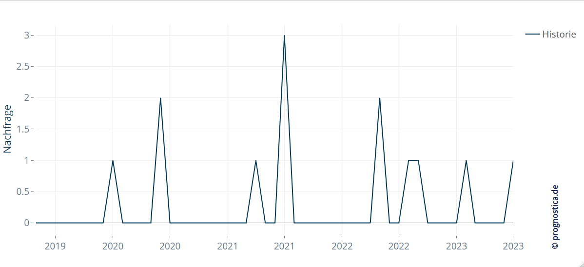
Forecasting for demand planning tends to be easier when volumes are high and patterns are regular. If there is a large customer base involved, it helps to balance out fluctuations to a certain extent. When focusing on items with a small customer base, however, you often see intermittent demand: in many of the time intervals considered (e.g., months or weeks), demand is 0 (= no demand); positive demand occurs only at the few remaining points in time. For such series, classical techniques like exponential smoothing often cannot estimate a model with clear trend and seasonal components.
From a producer’s point of view, it is often precisely these items that require good forecasts. Even a single order for a certain quantity of such an item can, under certain circumstances, affect the safety stock and potentially cause a temporary out-of-stock situation. Fortunately, there are specialized statistical procedures tailored to the specifics of intermittent demand.
Intermittent forecasts reflect the known pattern
A classic for intermittent demand is the Croston method. It models the expected demand size and the time between non‑zero demands separately and updates both over time. In forecasting, Croston assigns the expected demand to the specific future interval(s) in which it is – roughly speaking – most likely to occur.
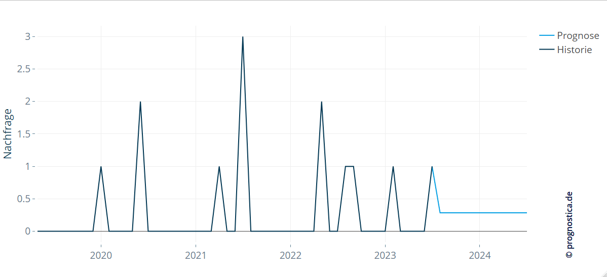
Averaged forecasts for intuitive planning
As an alternative to assigning demand to specific future points, a common Croston variant produces a smoothed forecast for intermittent demand. It combines the estimated sizes and inter‑arrival times and outputs an average demand for the next few intervals. Notably, it spreads the expected demand evenly across upcoming periods rather than distinguishing which specific week or month an order will occur.
This variant is the standard output of many planning tools supporting Croston. While the forecast looks quite different from the historical pattern, it often maps more naturally to regular production or procurement – which can make it more intuitive for planning than a spike‑like intermittent forecast.
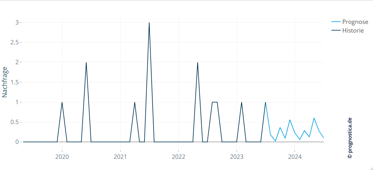
Between the extremes
Interesting insights lie between these two extremes. Here, the expected demand is neither purely intermittent nor fully even across periods. Instead, intervals with a higher probability of demand receive higher forecast values, while others receive less. One way to derive the weights is to model the discrete random variable “time to next demand” as a renewal process – events occur independently and follow the same distribution. By estimating this distribution from historical events, you can compute probabilities for future occurrences and obtain a forecast pattern that sits between a constant and a purely intermittent forecast.
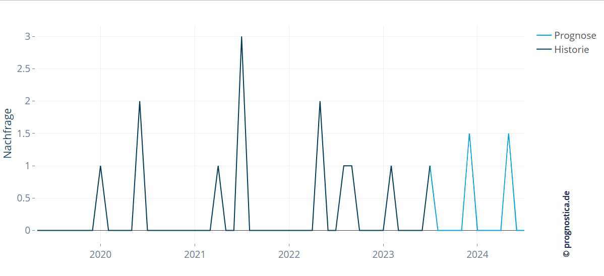
Pattern‑recognition methods capture more complex regularities
“From experience, there’s no demand in January. If there is, then there’s also an order in February – but definitely not in March.”
This fictitious rule illustrates a demand pattern that a simple annual seasonality component would not capture, even though certain months play a role in planning. Instead, future demand depends strongly on the type and extent of previous events.
To model such patterns, a broad range of machine‑learning methods can be used for forecasting. Techniques like decision trees (e.g., CART or Random Forests), support‑vector regression, or neural networks can uncover complex, non‑obvious patterns and project them forward. It is crucial to represent temporal dependencies appropriately via features; most ML models are not time‑aware by default. This requires sufficiently long histories so that models can learn the patterns, and careful selection of features that demonstrably influence demand. Cross‑validation adapted to intermittent series is very useful here.
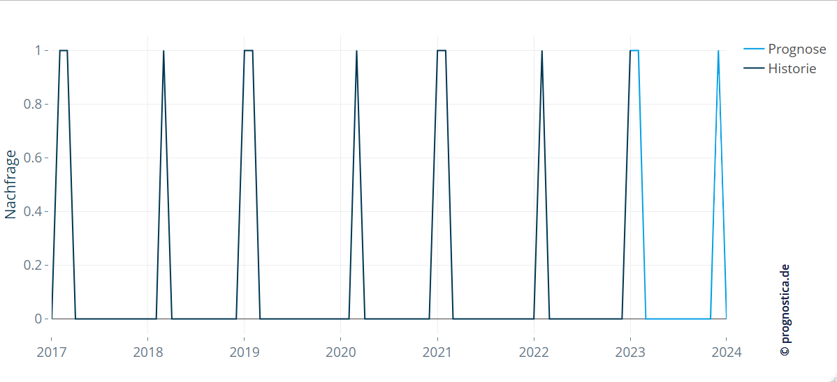
The figure below shows that the rule “if demand occurs in January for a spare part, there will also be demand in February” was detected and correctly forecast in the example.
Using additional information for intermittent demand
In many cases it is beneficial to provide forecasting models with additional information beyond the item’s own history. This is particularly helpful when only a short history is available, where complex statistical or ML models are hard or impossible to fit. By enriching simpler statistical approaches with informed assumptions, you can often obtain meaningful results even from limited data.
Example assumption: “If there is a pattern, it repeats every 12 months.”
Especially with very short histories, incorporating available knowledge and integrating it properly into the model becomes increasingly important – for example, known annual seasonality. Product‑related knowledge is often maintained in the company or known by staff (e.g., planners, sales).
Examples of useful information for forecasting spare parts include:
- Known seasonal effects
- Product lifecycle stage
- Predecessor and/or successor products
- Hierarchical context (e.g., base product vs. processed article)
- Open orders
- Customer inactivity information
- External indicators
To leverage such information, you typically need case‑specific data joins and appropriate forecasting methods. A dedicated article on “Small Data” discusses challenges and options for working with limited data in more detail.
At the beginning and end of the product lifecycle: an example
Most items have a finite production lifecycle. At the beginning (launch) and at the end, forecasts based solely on the item’s own history can quickly become inaccurate – e.g., if demand rises rapidly shortly after market introduction. Accurate demand and inventory forecasts may critically depend on lifecycle information.
For reliable forecasts of an item that is still at the beginning of its life cycle after its introduction and therefore has a very short data history, it can be advantageous to use data histories of items that have similar characteristics to the one being examined. By using the known history of similar items as an influencing factor in the prediction model for the item in question, the new prediction model can adopt some of the patterns seen in the old history. For products with short lifecycles (e.g., a smartphone maker’s yearly models), chaining predecessor and successor products can substantially improve forecast quality. At the end of life, caution is required as well: even if a successor exists, the original item may still see residual demand that tapers off. Here, adjusting the base forecast via suitable features or an explicit phase‑out component can align it with the expected decline.
Selecting the right method
We’ve seen that good forecasts for intermittent demand are important – and that there are many candidate techniques. How do you choose the right one for your data?
In practice, you select a set of plausible candidates first. Don’t neglect domain expertise about the product, its specifics, lifecycle phase, and potential explanatory variables. Used well, this knowledge enriches algorithms and improves practical usefulness.
Quantitatively, evaluate candidates by backtesting on a sufficiently long past period for the specific forecast object (e.g., demand for an item). Consider the best‑performing techniques for production use. Additional criteria may be relevant depending on the case and method family and can influence the final choice.
An important question: what does “best” mean? Which metrics should quantify performance? You can use error/accuracy metrics that compare forecasts to realizations. Our article on forecast accuracy provides an introduction and discusses measures such as PIS or SPEC that are tailored to intermittent time series.
Quantifying uncertainty
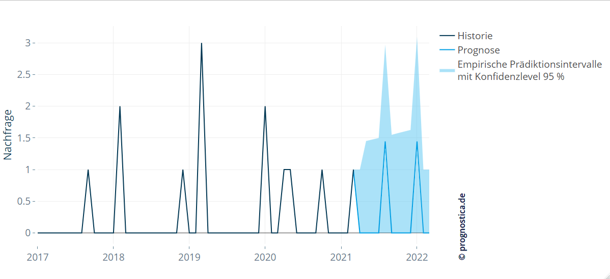
No matter how good a forecast is, it will differ from reality to some degree. Therefore, for intermittent series it’s also important to assess uncertainty in addition to point forecasts (e.g., to plan appropriate safety stocks). Many statistical methods provide prediction variance directly. Where model‑based variances are not available – e.g., in the pattern‑recognition approaches above – you can fall back on empirical variance given a sufficiently long history (e.g., to compute MAD). The validation mechanisms mentioned above yield useful estimates. Visualizing uncertainty via prediction intervals works well – though for intermittent series intervals can become quite wide.
The takeaway: solid forecasts for intermittent time series
Good demand forecasts are essential for planning: they help avoid excess stock and out‑of‑stocks. For products with intermittent demand or short, dynamic lifecycles, the choice of methodology matters even more. Enriching the item’s history with additional information and integrating it into the forecasting approach can significantly improve results – enabling accurate and automated planning even for intermittent demand.
Eager to generate forecasts for your own intermittent data?
Try our forecasting software future.