How to Measure Forecast Accuracy – Best Practices

If you want to use data to look into the future and create forecasts, it makes sense to follow well-established scientific standards. But how good will the forecasts be in your specific case? That’s hard to say upfront. This article outlines best practices for evaluating forecast accuracy in practice.

Even before a project starts, we’re sometimes asked: “What forecast accuracy can you achieve?” – before we’ve even seen any data. As much as we’d like to give a number, the only sensible answer is: “We’ll know once we’ve tried.” Every use case is different. On very granular levels (e.g., weekly material demand per SKU), accuracy is often lower than on aggregated levels (e.g., monthly revenue for a business unit). Claiming upfront “we can reach 92%” would be guesswork. We may have an informed expectation based on similar projects – but certainty usually only comes after testing on your data.

It’s also not just about sophisticated methods and techniques. The inherent volatility of the phenomenon determines how predictable it is. And accuracy can change over time. Periods of elevated uncertainty typically make it harder to achieve the same accuracy as in stable phases.

Forecast accuracy as the counterpart to error metrics

So, we need to quantify accuracy. A gut feeling then becomes a robust belief about predictive quality. You can compare different techniques and vendors and get a realistic sense of what’s achievable in your case. Because creating forecasts isn’t the end of the story.

There are best-practice approaches to measuring forecast accuracy. However, as hinted: different use cases may warrant different computation methods.

There are two temporal perspectives for judging forecasts:

1. Live: track how forecasts perform in production. This is often called forecast monitoring.
2. Retrospective: evaluate how a technique or model would have performed if applied in the past. This backtesting step is typically performed before going live and is crucial for selecting models and strategies.

The forecast error measures deviation

Whether you assess forecasts retrospectively or live, the same principle applies:

1. From a given point in time, generate a forecast for a future time point.
2. Observe the realized value at that future time point. In monitoring, you wait until it occurs; in backtesting, it’s already known.
3. Compare realized value with the prior forecast. The difference is the forecast error.

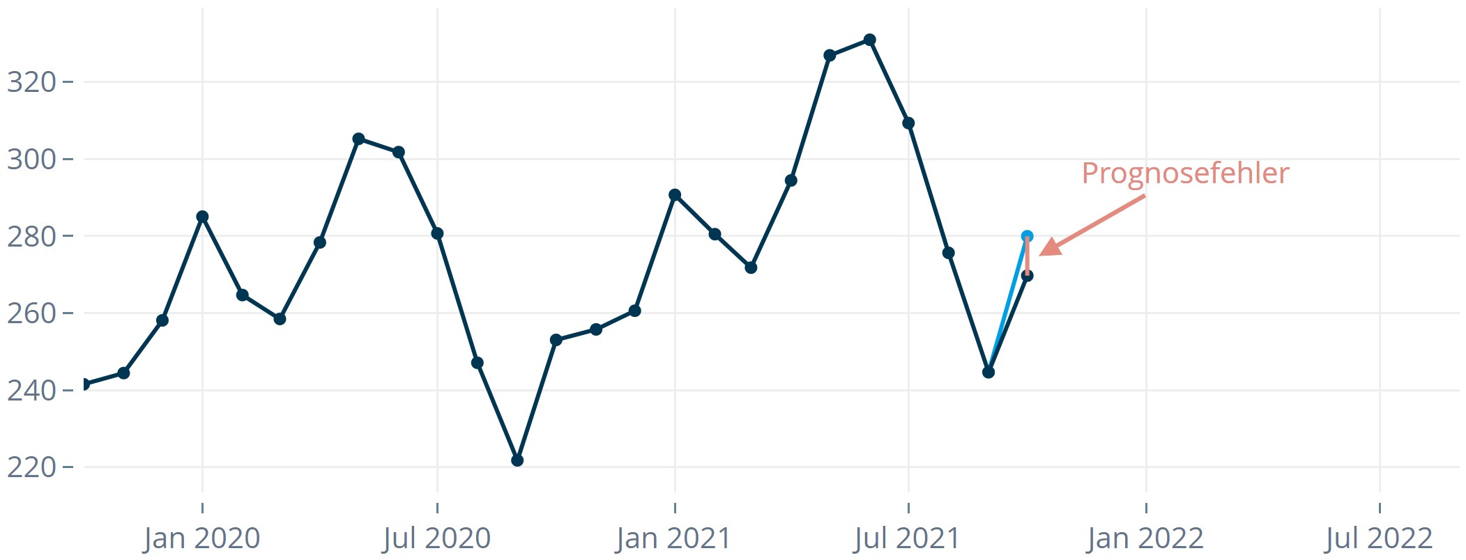
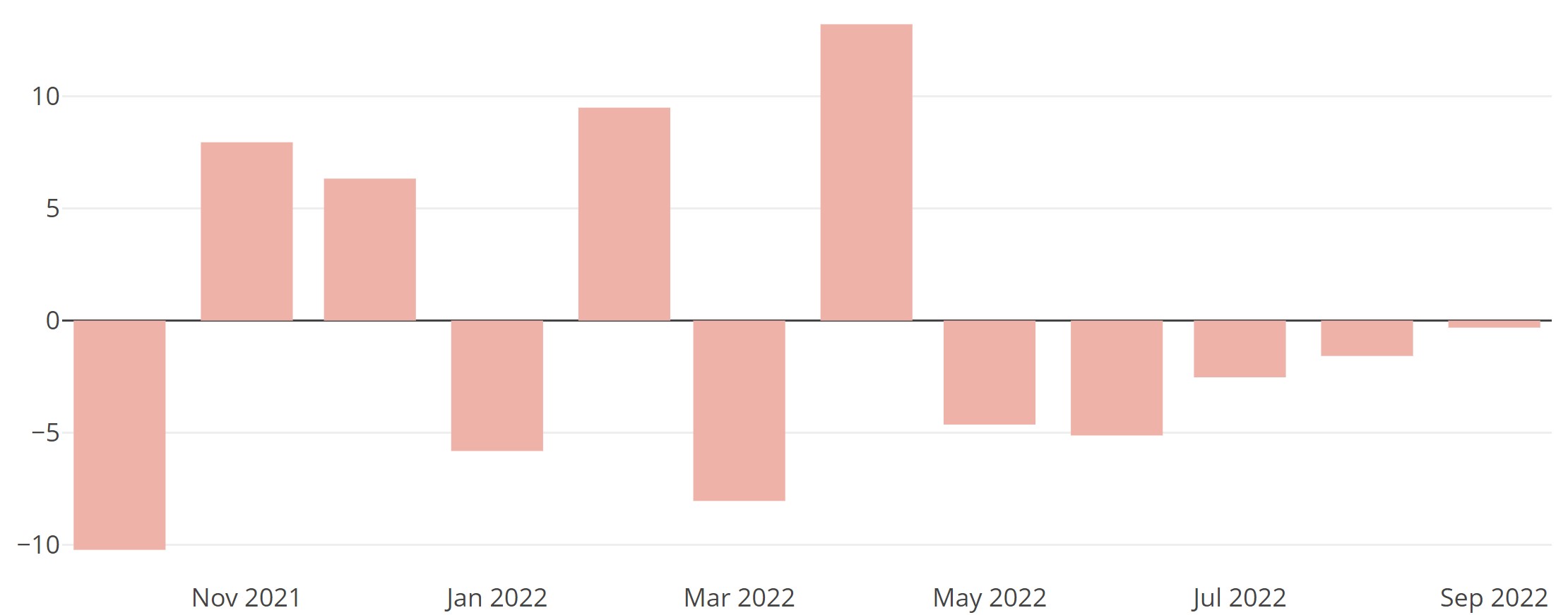
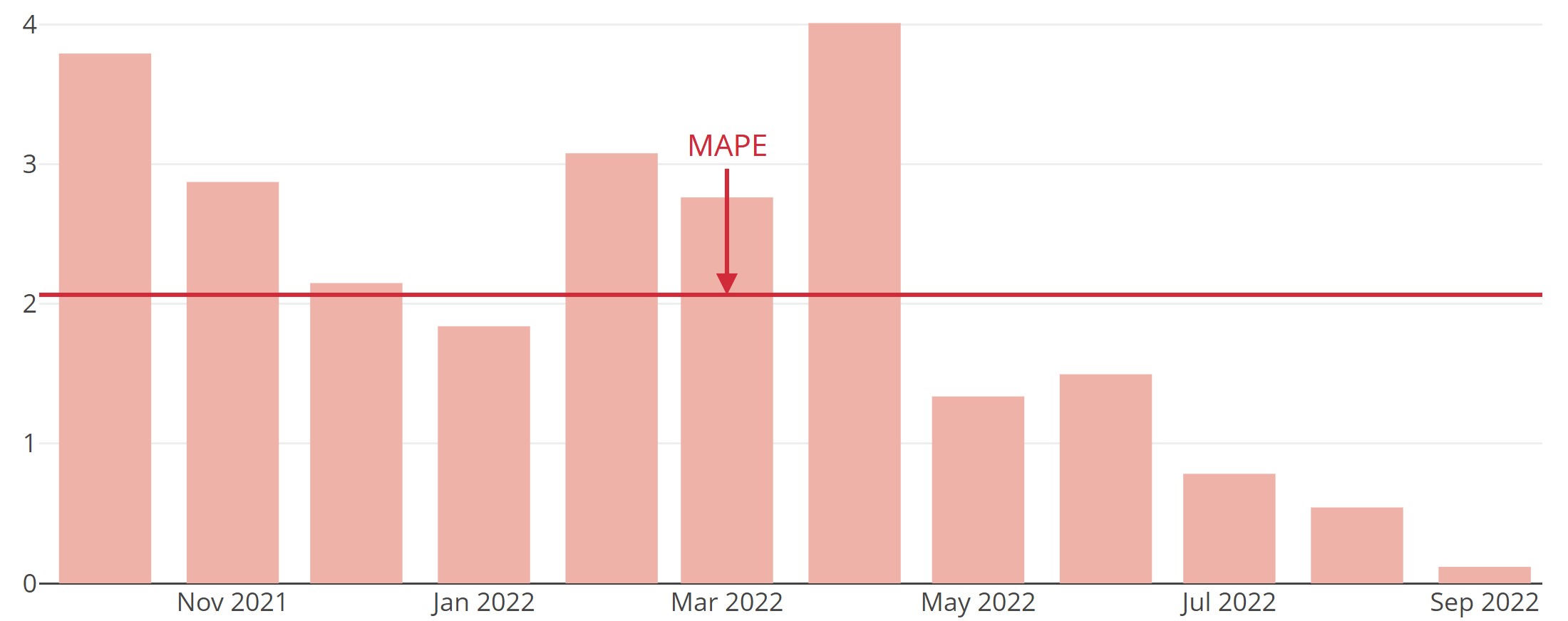
The forecast error at time i – the difference between the actual value (act_i) at time i and the forecast (fc_i) for time i – is the basis for most metrics used to evaluate forecast quality.

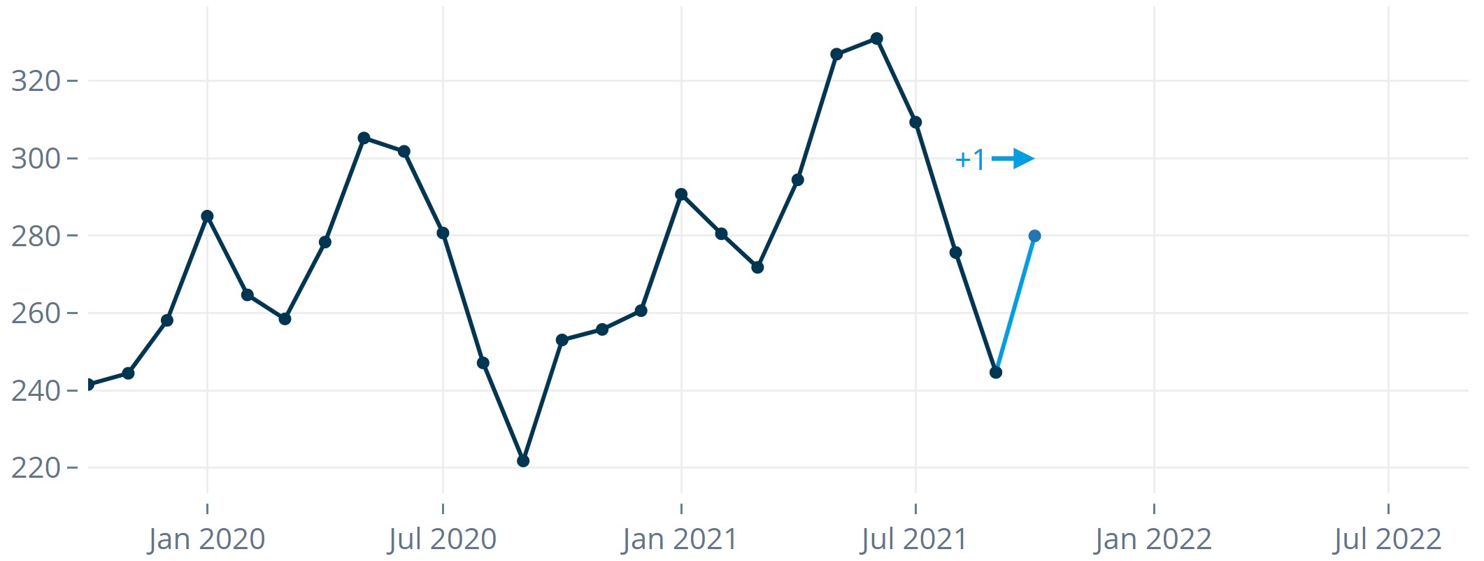
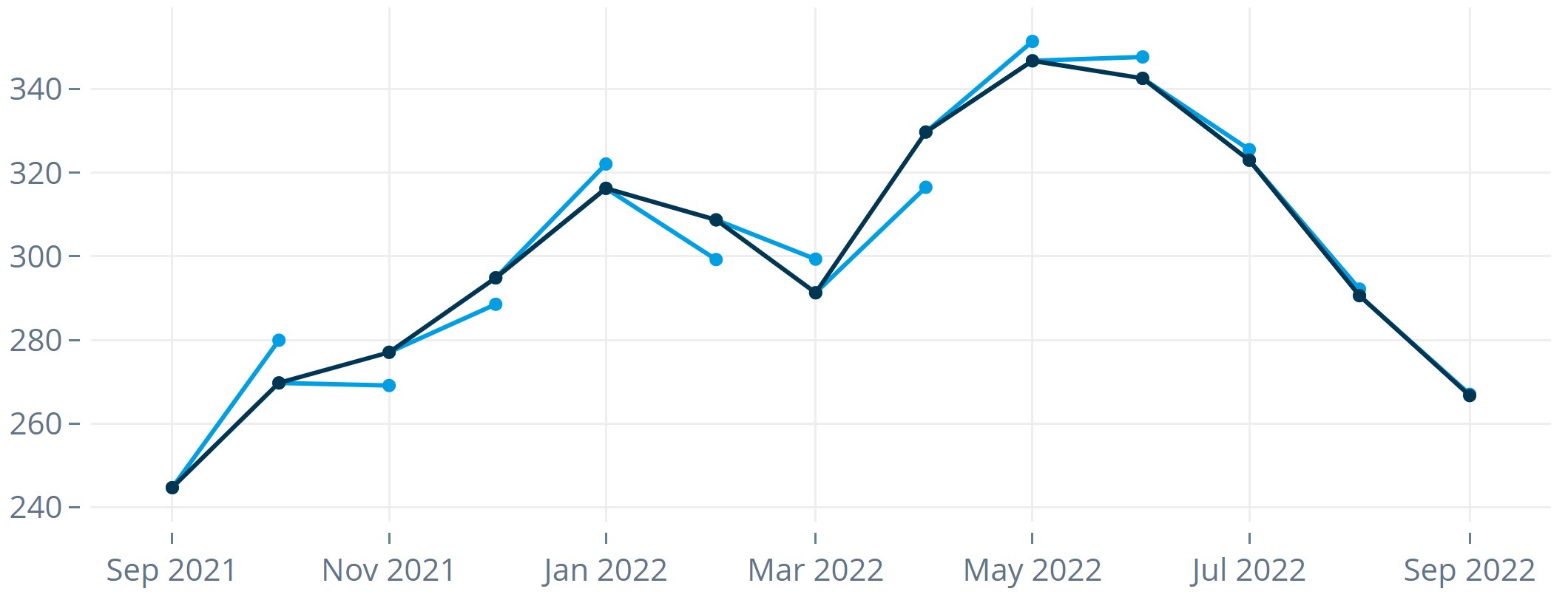
The error shown in Figure 1 is a 1-step forecast error. It is based on 1-step forecasts, i.e., from a given time you look exactly one interval ahead (e.g., one month). You can also evaluate higher forecast horizons. For example, by the end of July many companies have already finalized the plan for August. Instead, October is now in focus – the 3-step-ahead forecast becomes particularly relevant. In that case, you would emphasize evaluating the 3-step error and optimize accordingly.

The following metrics can be computed for 1-step as well as higher-step forecasts.

Backtesting: Hindsight makes you wiser

To gain a reliable view of your forecasting strategy, you don’t evaluate a single time point but a longer period. In backtesting, you simulate forecasts for a past period, e.g., the last 12 months. You can then leverage the fact that actuals are known and compare them to forecasts. In a time-series context, the process essentially is:

1. Split the historical data into a training period and a test period (backtest window).

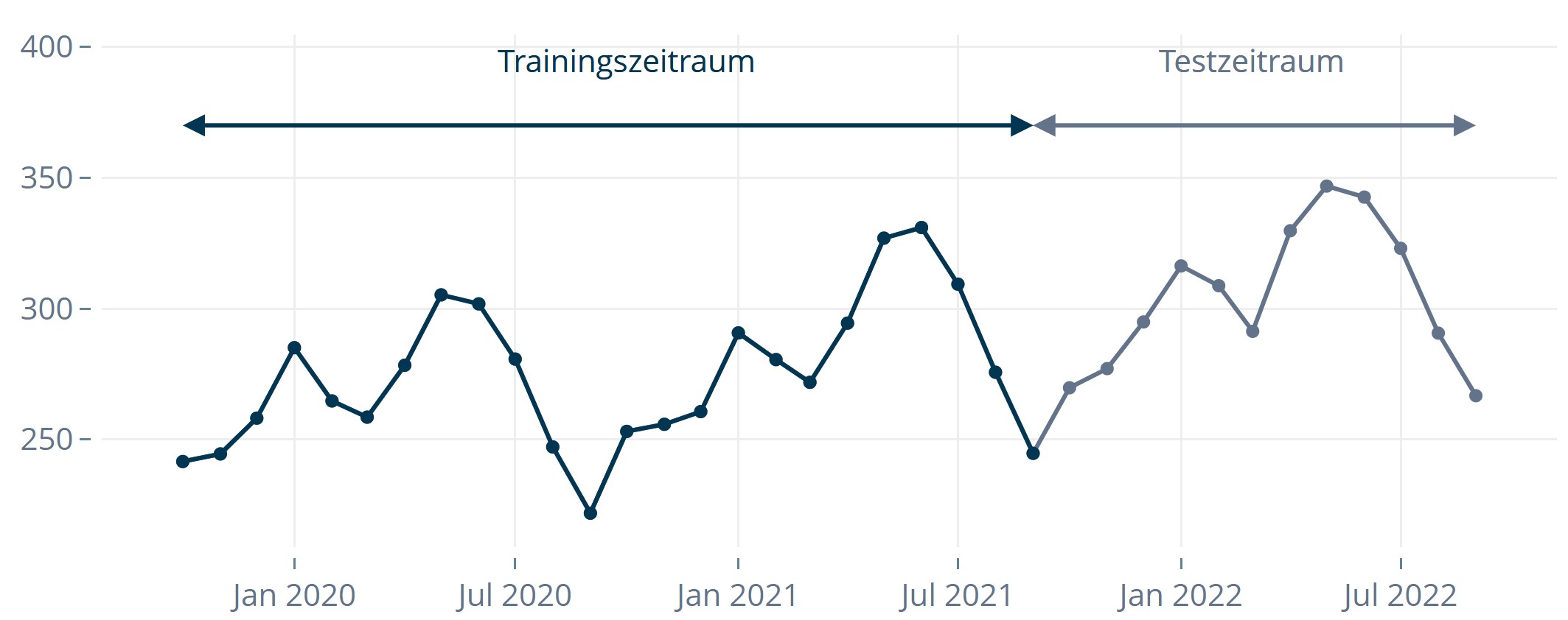
2. Create a forecast for the first time point in the test period, pretending you only know observations up to that point.

3. Then forecast the second time point in the test period, again using only information available up to then.
4. Continue until the end of the test period.

5. Compute the forecast errors for all time points in the test period.

6. Aggregate the errors (and possibly forecasts) into an informative summary metric. This yields an error measure indicating how well or poorly the forecasts performed.

Error metrics summarize forecast errors

There are many ways to evaluate models using error or accuracy metrics – most rely on analyzing forecast errors. We’ll introduce selected metrics rather than an exhaustive list, highlighting different categories and use cases. The same metric may be very appropriate in one context and entirely unsuitable in another.

Below, we describe error measures that quantify how bad a forecast is, not how good. Forecast accuracy is the positively phrased counterpart. Some compute accuracy as 100%−MAPE (see below). We focus on error measures where “the closer to zero, the better.”

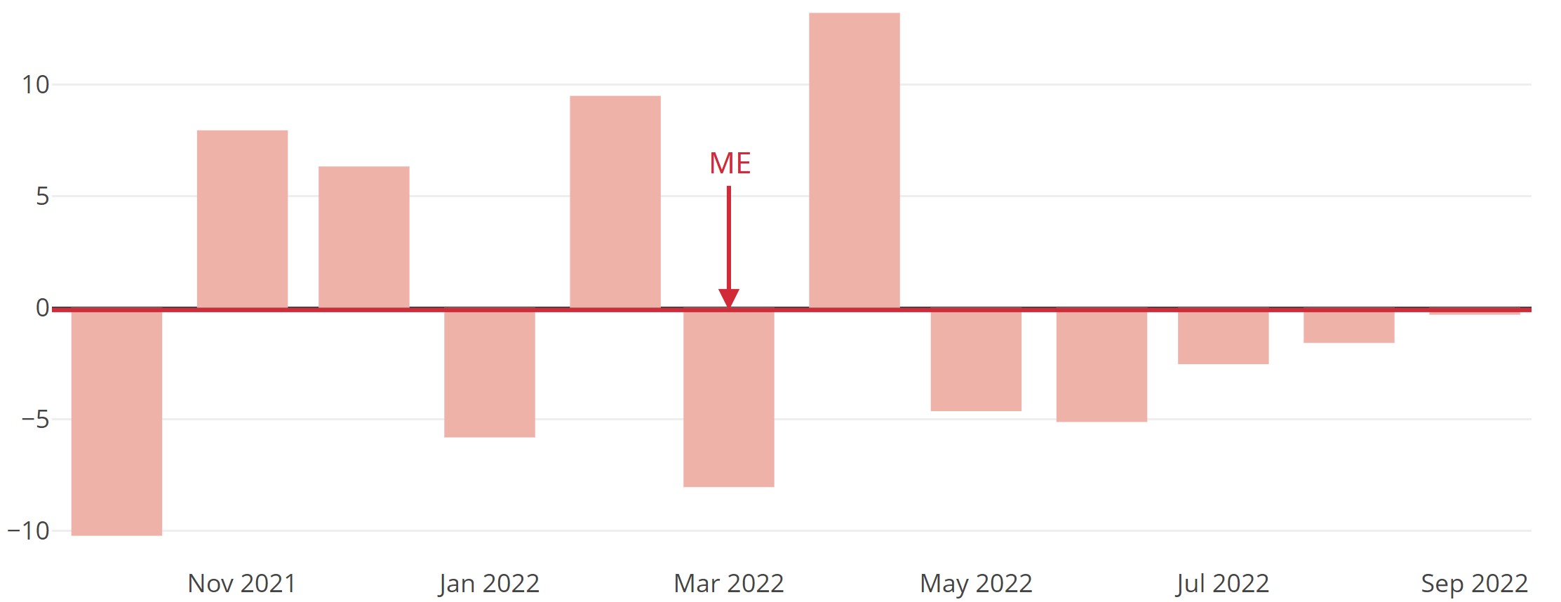
ME (Mean Error)

The most straightforward measure averages the n forecast errors over the backtest window.

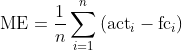
ME is sensitive to the sign of errors. If it’s below zero, on average you underestimated; above zero, you overestimated. In the extreme, if half of the actuals were underestimated by x and the other half overestimated by x, ME is zero – even though forecasts were potentially far off at every time point.

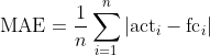
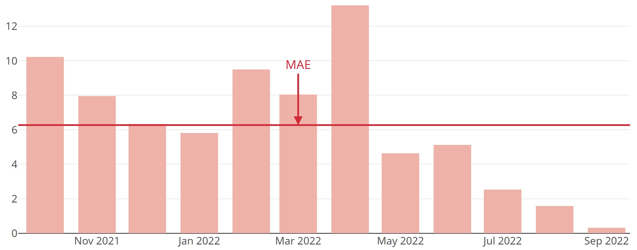
MAE (Mean Absolute Error)

To avoid cancellation between over- and under-forecasting, MAE averages the absolute forecast errors.

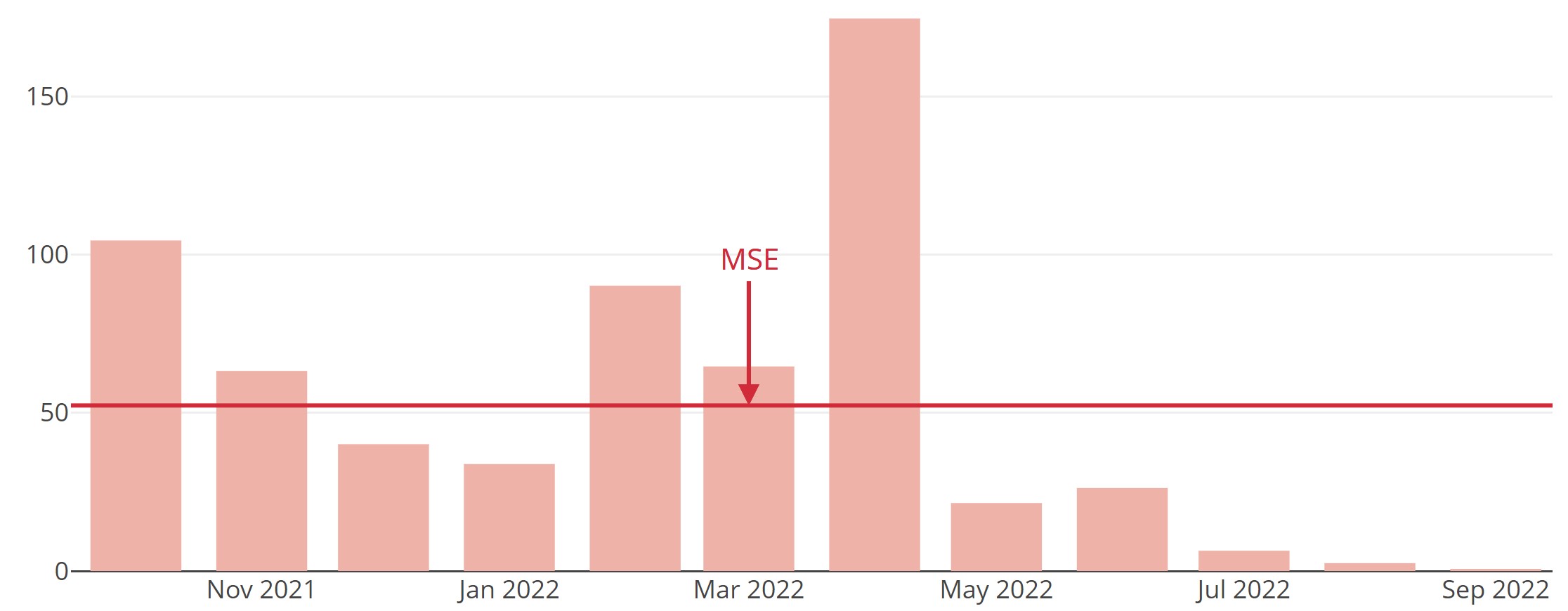
MSE (Mean Squared Error)

If you want to penalize large errors more strongly than small ones, square the errors before averaging – yielding MSE.

Squaring also removes the sign. MSE is one of the most widely used measures in forecasting and statistics (e.g., as a loss for linear regression). Note that squaring makes MSE more sensitive to outliers than MAE.

Instead of MSE, many report RMSE (Root Mean Squared Error) to bring the unit back to the original scale (e.g., EUR instead of EUR²).

MAPE (Mean Absolute Percentage Error)

Raw errors and metrics like ME, MAE, MSE are not scale-free. A deviation of 100 units might be acceptable when typical volumes are in the tens of thousands, but not when they are in the tens or hundreds. To compare across scales, MAPE evaluates errors relative to the actual values: first compute percentage errors, then take absolute values and average.

PIS (Periods in Stock)

Periods in Stock (PIS) sums up how long forecast errors remain as stock in a hypothetical inventory until they are offset by errors in the opposite direction. Here, the direction of the deviation matters.

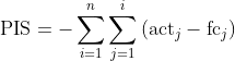
PIS also considers the duration of the mismatch between forecast and actuals – which the above measures do not. It’s well-suited for intermittent time series with many zeros, common when analyzing demand at very fine granularity. This typically applies to inventory contexts with non-negative values. MAPE is not suitable here because you would divide by zero. PIS was introduced by Wallström and Segerstedt (2010).

Example: A forecast that occurs several days too early (Forecast 1) results in a higher PIS (worse accuracy) than a forecast shifted by one day (Forecast 2), while other metrics like MAE rate both cases equally:

Higher forecast horizons often matter more than short ones

In model building, 1-step errors often receive the most attention. In practice, however, higher-step horizons are frequently more relevant. Many companies care about more than one horizon simultaneously. In such cases, it can make sense to aggregate error metrics across multiple horizons. Which horizons to emphasize and how to aggregate is highly use-case specific and depends on processes and planning cycles.

Example: A company typically plans production with a lead time of 3–4 months. The 1- and 2-step forecasts are less relevant because actions are already locked in. Forecasts for three and four months ahead are crucial. In this case, a weighted mean of the RMSE for the 3- and 4-step forecasts may be the right evaluation metric.

Choose a metric that fits the use case

Every company and use case is a bit different. For intermittent demand, MAPE is not applicable. Conversely, PIS is not suitable for highly aggregated time series without zeros. Planning processes also differ – so the “right” metric varies.

Whether you are a data scientist or a business user: asking about forecast accuracy is always worthwhile. If you observe, review, and question your forecasts, you gain confidence, learn, and can improve your strategy if needed. As a user, you gain solid numbers for management and benchmarks for comparison.

If you want a more qualitative checklist, see our article 10 Characteristics of a Good Forecast — covering benchmarks, transparency, prediction intervals, reliability, and more.

References

• Wallström, P., Segerstedt, A. (2010). Evaluation of forecasting error measurements and techniques for intermittent demand. International Journal of Production Economics 128(2), 625–636.

Do you wonder what forecast accuracy is achievable for your use case and data? Try it out for free with the forecasting software future!